Optimo has been updated since the time that this blog post was published. Please see the most Updated information about Optimo here (https://github.com/BPOpt/Optimo/wiki/0_-Home). This blog post demonstrates the older version of Optimo.
Optimo is a multi-objective optimization tool that enables Dynamo users to optimize problems with single and multiple objectives using evolutionary algorithms. The current version of Optimo uses an NSGA-II (Non-dominated Sorting Genetic Algorithm-II), a multi-objective optimization algorithm to reach to a set of optimal solutions. More optimization algorithms will be added to Optimo soon. Optimo is developed by Mohammad Rahmani Asl and Dr. Wei Yan in the BIM-SIM Lab at Texas A&M University using jmetal.NET open source code. Optimo source code is available on Optimo Github. The latest version of Optimo is available as a package in Package Manager. The package comes with all the necessary files (custom nodes and .dll files) to run Optimo along with a few Dynamo samples that can be used to start working with Optimo. You can find the Dynamo samples in the folder (named Packages/Optimo/extra) in the Dynamo packages directory (more on folder locations here). Optimo requires the Dynamo daily build 0.7.4.3192 or a newer version. In the process of design optimization, in many cases, designers need to solve problems with multiple conflicting criteria. For these so called multi-objective optimization problems, it is not always possible to find one optimal design solution that satisfies all design objectives. There are two common approaches to multi-objective optimization problems:
- Simple Aggregation
- Pareto Optimal
In simple aggregation, a composite objective function is defined by combining all of the individual objective functions. The composite objective function can be determined with various methods, such as the use of weighting factors. Determining the composite objective function needs knowledge of the relationships among individual objectives and their weighting factors and not always possible. The second approach seeks a set of promising solutions, known as a Pareto-optimal set, given multiple objectives. Pareto Optimality supports decision making by finding the equally optimal solutions such that it is not possible to improve a single individual objective without causing at least one other individual objective to become worse off. Optimo enables you to optimize multiple objectives in Dynamo and to find the Pareto Optimal for the defined problem. The following two simple examples are provided to demonstrate how you can set single and multiple objective routines in Dynamo. You can find the Dynamo files for these examples in the Packages/Optimo/extra folder after Optimo is installed.
Example 1 – Minimum Z Value on a Surface (Single Objective) This example shows the process of setting up Optimo for single objective optimization. The objective of this example is to find a point on a surface with the minimum Z value. The parametric variables are X and Y of the points.  The user can modify population number, lower and upper limits of optimization variables, and the number of objectives (it is one for the single objective optimization). The “NSGA-II.InitialSolutionList” node creates a list of random numbers (the size of which is the population size) for each variable (initial population list) within the specified range. The population list includes a placeholder for fitness function results which will be assigned when the fitness function results are evaluated. The number of variables can be changed by adding or removing an index to the “List.Create” node (both upper and lower limits must have the same number of indices). The output of the “NSGA_II.InitialSolutionList” node is a list of lists—lists of variables and objectives. Optimo is designed in a way that the user can modify the fitness functions without needing to change to the whole process or to write any script. A list of variables can be taken from the initial list of populations and can be used as an input to the defined fitness functions. Objective functions can be added and removed, but the “number of objectives” input must match the number of objective functions.
 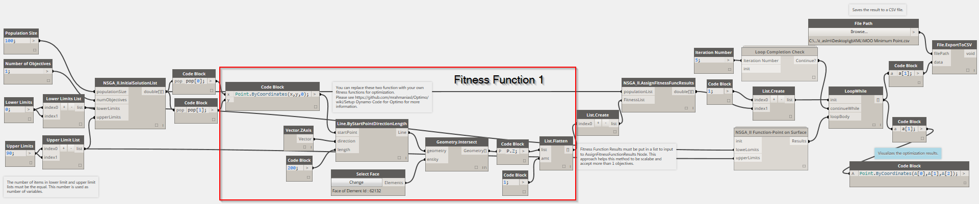 The two lists of variables created by InitialSolutionList are used as X and Y values to create a range of points on the XY plane. Then they are projected to the surface by shooting rays toward the surface. The Z values of the intersection points are gathered as the result of the fitness function. The “NSGA-II.AssignFitnessFunction” node assigns the fitness function values to the population list.
  The Dynamo graph below is contained inside the “NSGA_II.Function Point on Surface” custom node. The function of this node is to run the NSGA II algorithm recursively to generate the specified number of generations. The first input to this custom node, “init” is a list containing two elements. The first element in the list is the counter that controls the number of iterations. The second element is the population of the previous generation. This gets fed into the “NSGA_II.GenerationAlgorithm” as an input along with the lowerLimits and upperLimits (which serve the same purpose as in the main Dynamo file).
  The GenerationAlgorithm function creates a new population based on the previous generation. This new generation is then evaluated with the same fitness functions as in the main Dynamo file, and the fitness function results overwrite the objectives’ values in this new generation. The “NSGA_II.Sorting” node takes the previous generation as well as the current generation, and ranks them in the equally optimal solution front based on their fitness (best results first). The “LoopWhile” node is essentially running in the “NSGA_II Function” node recursively. The number of loops depends on the iteration number inserted into LoopCompleteionCheck as an input. The init input gets incremented by one in each loop, and once init reaches the same value as completionCheck, the loop ends and the Dynamo program continues. The LoopBody input is the output from the NSGA_II function (it becomes the input for the recursive call to the NSGA_II Function node).
Example 2- Minimizing SCH Test Function (Multi-Objective Optimization) This example shows the setup for a simple multi-objective optimization algorithm. This example uses the SCH test function optimization problem—Schaffer function N.1 Test_functions_for_optimization. For a more complex example using Optimo see BIM-based Parametric Building Energy Performance Multi-Objective Optimization. The test functions are useful to evaluate the optimization algorithm. The SCH test function tries to minimize two conflicting objectives as demonstrated in the image below. When trying to minimize one of the fitness functions, the other function value increases. You can replace the SCH fitness functions to create your own optimization problem.  The Dynamo graph for the SCH test function is provided in the image below. As you can see the number of objectives is changed to two to match with the SCH problem definition. The results of fitness function 1 and 2 are put into a list using “List.Create” node to be inserted into the “NSGA-II.AssignFitnessFunctionResults”.
 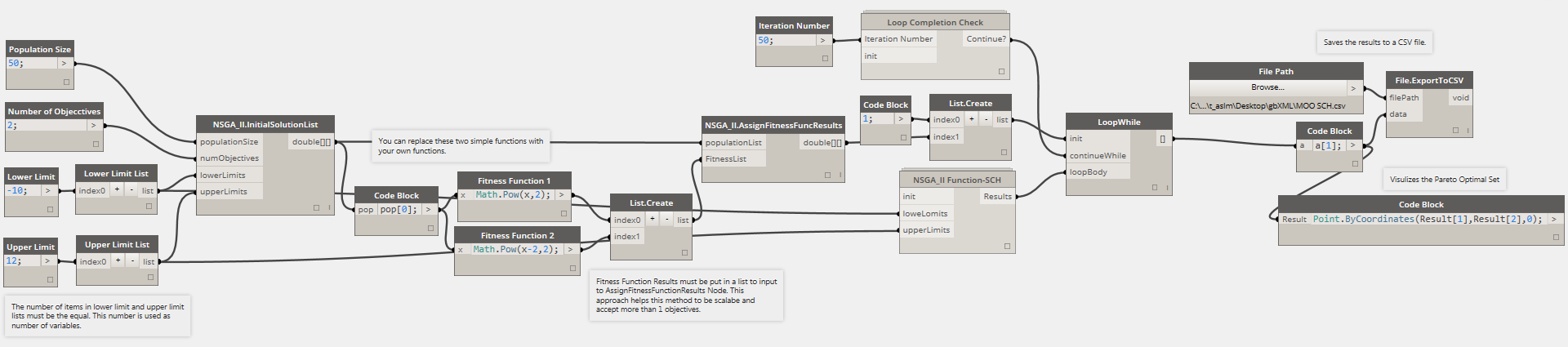 The “NSGA-II Function” custom package is changed accordingly to match the main Dynamo graph for the SCH example. You can see the graph of this custom package below.
 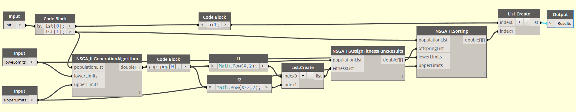 As mentioned before, there are multiple optimal solutions (Pareto Optimal solutions) for contrasting objective functions. The image below shows a set of best solutions for the SCH test.
Acknowledgments We would like to thank Dynamo team, Saied Zarrinmehr and Alexander Stoupine at Texas A&M University for their contributions in this project. This research project is partially supported by the National Science Foundation under Grant No. 0967446.
——–Mohammad Rahmani Asl is a PhD Candidate in the Department of Architecture at Texas A&M University. He has been working as a Ph.D. Researcher for the Autodesk Building Performance Analysis team for the past few months. He has a lot of experience in Building Energy Simulation and optimization (mrah-at-tamu.edu). Dr. Wei Yan is an Associate Professor in the Department of Architecture, Texas A&M University. His academic interests include Computer-Aided Architectural Design, Parametric Modeling, Building Information Modeling, Building Science, Simulation, and Optimization.